Squeezing Performance from the Redshift Giant

12/30/2025

Squeezing Performance from the Redshift Giant

Preface

This (very long overdue) blog post marks the beginning of my data engineering series (!), where I document my learnings and experiences with modern data infrastructure. In this first part, I share my deep dive into Amazon Redshift, where I explore its architecture, internals, and optimisation techniques that I applied to improve storage efficiency and query performance on production systems.

Introduction

Starting my internship at GovTech Singapore, I was tasked with identifying and optimising inefficiencies in the organisation’s Amazon Redshift data warehouse. This central data platform served as the backbone for analytics and reporting across multiple teams, making performance and cost optimisation critical priorities.

My initial task was to explore the Redshift cluster, understand its workload patterns, and identify opportunities to optimise storage and reduce query latency. With almost no prior experience in OLAP databases, I embarked on a learning journey that would fundamentally shift how I think about data systems.

Setting the Scene: The Learning Journey Begins

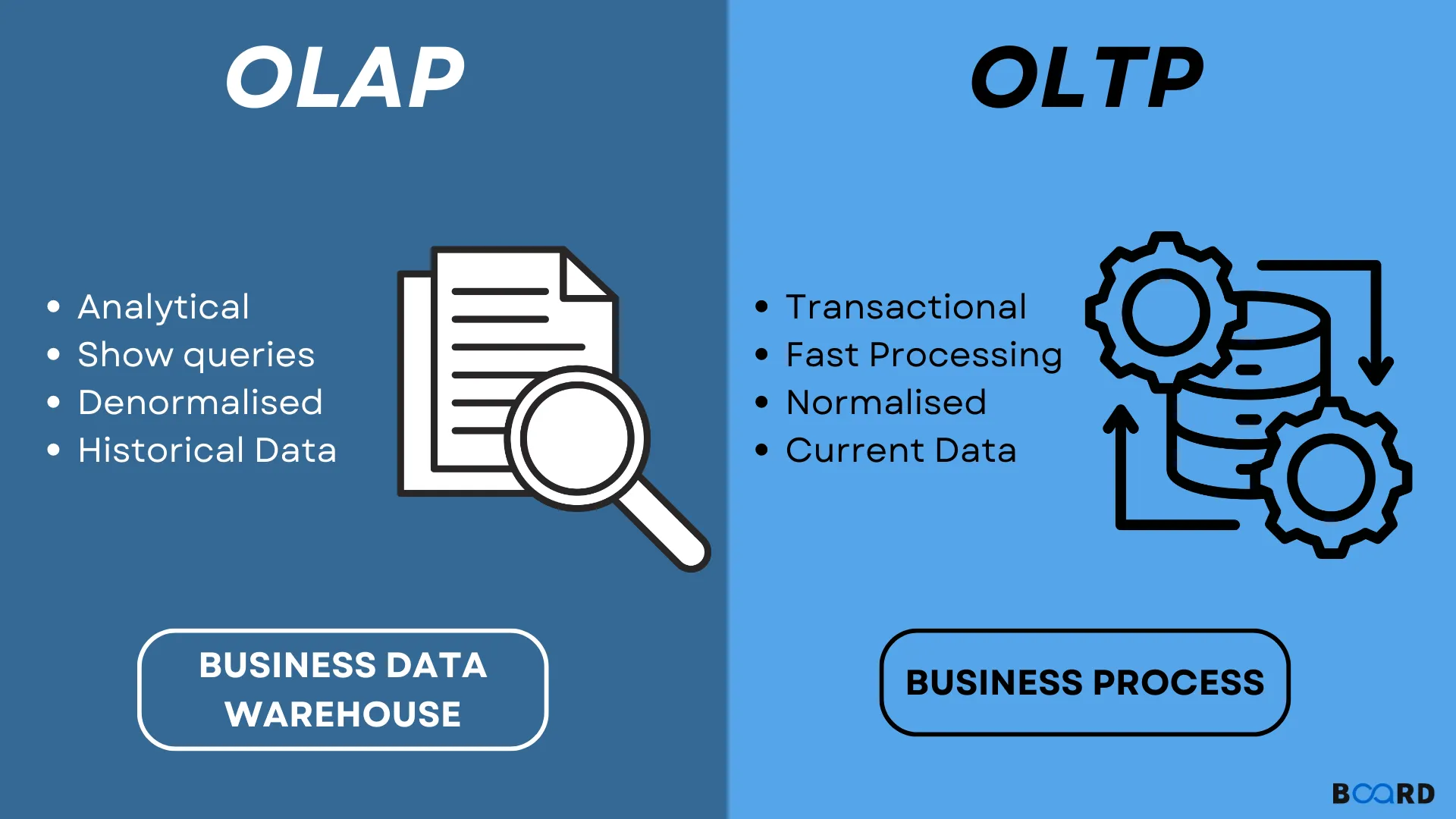
Walking into this role, my database knowledge was primarily rooted in traditional OLTP (Online Transaction Processing) systems such as MySQL or PostgreSQL. These databases excel at handling frequent, small transactions with strong ACID guarantees. But Redshift operates in a completely different paradigm.

My first week involved extensive reading, documentation deep-dives, and hands-on exploration. One resource that proved invaluable was Max Ganz II’s blog series on Redshift Observatory, particularly his post: “Introduction to the Fundamentals of Amazon Redshift”. It was through this guide that laid the groundwork for my understanding of Redshift’s architecture and design philosophy.

Some of the key topics I needed to master:

• Row-store vs Column-store architectures
• Sorted vs Unsorted data
• Cluster architecture and disk management
• Query compilation and execution
• System design principles for analytical workloads

OLAP vs OLTP: Understanding the Paradigm Shift

Why Redshift is the Chosen Tool for Analytics:

1. Columnar Storage: Instead of reading entire rows (which includes data you don’t need), it only reads the specific columns you ask for.
2. MPP (Massively Parallel Processing): It splits a giant query into tiny pieces and runs them simultaneously across dozens of “worker” nodes.
3. Modern Scalability: With RA3 nodes, we can scale compute (how fast it thinks) and storage (how much it remembers) independently.

Deep Dive: Redshift Internals

Row-Store vs Column-Store

Traditional databases store data row-by-row:

Row 1: [ID=1, Name='Alice', Age=30, City='Singapore']
Row 2: [ID=2, Name='Bob', Age=25, City='Tokyo']

Redshift uses columnar storage, storing each column separately:

ID Column:   [1, 2, 3, ...]
Name Column: ['Alice', 'Bob', 'Charlie', ...]
Age Column:  [30, 25, 28, ...]
City Column: ['Singapore', 'Tokyo', 'Seoul', ...]

• Analytical queries often read only a subset of columns, Columnar format reads only necessary columns, dramatically reducing I/O.
• Similar values in columns compress better (e.g., many ‘Singapore’ entries)
• Enables vector processing for faster aggregations

Sorted vs Unsorted Data

Redshift allows us to define sort keys on tables, physically ordering data on disk. This has profound implications:

Sorted data benefits:

• Zone maps can skip entire blocks during queries
• Range-restricted queries become much faster
• JOIN operations benefit from co-located data

Unsorted data challenges:

• Full table scans required more frequently
• Higher I/O overhead
• Degraded performance over time as data accumulates

Cluster Architecture

A Redshift cluster consists of:

• Leader node: Query coordination, query planning, result aggregation
• Compute nodes: Parallel query execution, data storage
• Node slices: Each compute node divided into slices (parallelism unit)

Understanding this architecture helped me optimize query distribution patterns and identify bottlenecks.

Core Optimization Concepts Explored

1. Cluster Management

Managing a Redshift cluster involves:

• Node selection: Dense compute (DC) vs Dense storage (DS) vs RA3 nodes
• Cluster sizing: Balancing performance vs cost
• Resizing strategies: Classic resize vs Elastic resize vs Snapshot-restore
• Maintenance windows: Scheduling for minimal disruption

Key learning: RA3 nodes with managed storage offer the best flexibility for growing datasets, separating compute from storage scaling.

2. Zone Maps

Zone maps are metadata structures that track min/max values for each 1MB block of columnar data. When a query filters on a column, Redshift uses zone maps to skip blocks that can’t possibly contain matching data.

Example:

SELECT * FROM orders WHERE order_date >= '2024-01-01';

If data is sorted by order_date, zone maps allow Redshift to skip all blocks containing only 2023 data, drastically reducing I/O.

Optimization insight: Choose sort keys that align with common query filter patterns.

3. Data Sorting

Redshift offers two sort key types:

Compound Sort Keys:

• Multiple columns sorted hierarchically (like a phone book: last name, then first name)
• Best for queries filtering on sort key prefixes
• Most common choice

Interleaved Sort Keys:

• Equal weight to all columns in sort key
• Better for queries filtering on different columns
• Higher maintenance cost (VACUUM slower)

My approach: Analyzed query patterns using system tables to identify most-filtered columns, then designed compound sort keys accordingly.

4. I/O Reduction: Columnar Format & Partitioning

Columnar storage inherently reduces I/O, but additional techniques amplify this:

Block-level compression:

• Each 1MB block is independently compressed
• Reduced disk space and network transfer
• Faster decompression than row-based formats

Partition elimination:

• While Redshift doesn’t have formal partitioning like traditional databases, sort keys create “virtual partitions”
• Combined with zone maps, this enables efficient data pruning

5. Column Encodings: The ENCODE AUTO Pitfall

Column encoding (compression) is critical for Redshift performance. Options include:

• RAW: No compression
• LZO: General-purpose compression
• ZSTD: Modern high-ratio compression
• Delta: For numeric sequences
• Run-length encoding: For repeating values
• Mostly encoding: For columns with few distinct values

The ENCODE AUTO problem: Redshift’s automatic encoding (ENCODE AUTO) analyzes initial data loads to choose encodings. However:

• It may choose suboptimal encodings if initial data isn’t representative
• Changes in data patterns over time can make initial choices inefficient
• Automatic encoding can’t be easily adjusted later without rebuild

Best practice: For critical tables, manually analyze data distributions and choose encodings explicitly, especially for large or long-lived tables.

6. Workload Management (WLM)

WLM controls query queueing and resource allocation. Key concepts:

Manual WLM:

• Define query queues with memory allocations
• Assign queries to queues based on user groups or query groups
• Configure concurrency per queue

Automatic WLM:

• Machine learning-based dynamic resource allocation
• Adjusts to query complexity automatically
• Easier management but less control

Configuration example:

Queue 1: ETL jobs (50% memory, concurrency 2)
Queue 2: Interactive dashboards (30% memory, concurrency 5)
Queue 3: Ad-hoc analysis (20% memory, concurrency 3)

Optimization: Match WLM configuration to actual workload patterns by analyzing query execution patterns in system tables.

7. Concurrency Scaling

Concurrency scaling automatically adds transient cluster capacity during traffic spikes:

• Burst clusters handle read queries
• Main cluster handles writes
• Billed per-second for additional capacity

When to enable:

• Unpredictable query spikes (end-of-month reporting)
• Mixed workloads with occasional bursts
• Cost-effective alternative to permanent over-provisioning

Tradeoff: Adds cost overhead, so analyze usage patterns to determine ROI.

8. Query Monitoring Rules (QMR)

QMR allows automated actions based on query metrics:

• Abort: Kill runaway queries exceeding thresholds
• Log: Record queries for analysis
• Hop: Move queries to different queue

Example rule:

-- Abort queries scanning more than 1TB
CREATE QMR abort_large_scans
WHEN query_temp_blocks_to_disk > 1000000
THEN ABORT;

Use case: Prevent poorly-written queries from consuming excessive resources.

9. VACUUM Commands

Over time, deleted rows and unsorted data degrade Redshift performance. VACUUM reclaims space and re-sorts data:

VACUUM types:

• VACUUM FULL: Reclaim space + re-sort (most comprehensive)
• VACUUM DELETE ONLY: Only reclaim deleted row space
• VACUUM SORT ONLY: Only re-sort unsorted data
• VACUUM REINDEX: Rebuild interleaved sort key indexes

Best practices:

• Schedule VACUUM during low-traffic windows
• Use VACUUM DELETE ONLY after large DELETE operations
• Monitor table unsorted percentage via SVV_TABLE_INFO
• Let auto-vacuum handle most cases; manual VACUUM for exceptions

10. SVV System Views

Redshift provides powerful system views for monitoring and optimization:

SVV_TABLE_INFO:

SELECT * FROM SVV_TABLE_INFO
WHERE schema = 'public'
ORDER BY size DESC;

Shows: table size, sort key columns, unsorted percentage, statistics, distribution style

Other useful views:

• SVL_QUERY_SUMMARY: Query execution details
• STL_QUERY: Query text and execution times
• SVL_QLOG: Query logging
• STL_LOAD_ERRORS: COPY command errors

Optimization workflow:

1. Identify large/frequently-queried tables in SVV_TABLE_INFO
2. Check unsorted percentage
3. Analyze query patterns in SVL_QUERY_SUMMARY
4. Adjust sort keys, encodings, or distribution keys accordingly

11. Zero-ETL Integration

A newer Redshift feature enabling direct integration with operational databases:

• Replicate data from Aurora, RDS, or DynamoDB to Redshift automatically
• No custom ETL pipelines needed
• Near real-time analytics on operational data

Benefits:

• Reduced engineering overhead
• Lower latency for analytics
• Simplified architecture

Limitations:

• Limited source database support (expanding)
• May not suit all transformation requirements
• Cost considerations for data transfer

Reflections: What I Actually Learned

Beyond the code and the SQL system views (SVV_TABLE_INFO became my most visited page), this internship taught me a core engineering truth: Optimization is a loop, not a one-time task.

1. Monitoring is Key: If you aren’t looking at the STL_QUERY logs, you’re just guessing where the bottleneck is.
2. Schema is King: You can have the biggest cluster in the world, but if your Sort Keys and Encodings are wrong, it will still feel slow.
3. Cost = Performance: Every byte saved is money stays in the budget. Optimization isn’t just about speed; it’s about efficiency.

This experience fundamentally changed how I approach data infrastructure. Moving from theoretical knowledge to hands-on optimization revealed the nuances and tradeoffs that textbooks can’t fully capture.

What’s Next?

This concludes Part 1 of my Data Engineering series. In the upcoming posts, I’ll cover:

• Part 2: AWS SageMaker Unified Studio
• Part 3: Data Lakehouse Architecture with AWS

Stay tuned for more data engineering deep dives!

Resources & References

• Max Ganz II - Redshift Observatory: Excellent series on Redshift fundamentals
• AWS Redshift Documentation: Official reference
• Redshift Best Practices: AWS optimization guide
• Redshift System Tables Reference: Essential for optimization

Thank you for reading! If you found this helpful or have questions about Redshift optimization, feel free to reach out.